Chapter 6 Model selection

Ref: here

In this section, we demonstrate how to compare the performance between different models. So the first step is to create a training and testing dataset.

library(C50)
data("mlc_churn")
table(mlc_churn$churn)/nrow(mlc_churn)

## 
##    yes     no 
## 0.1414 0.8586

We see that about 15% of the customers churn. It is important to maintain this proportion in all of the folds.

myFolds <- createFolds(mlc_churn$churn, k=5)
str(myFolds)

## List of 5
##  $ Fold1: int [1:1000] 4 9 18 25 30 33 42 47 67 73 ...
##  $ Fold2: int [1:1000] 1 3 5 11 14 23 36 44 55 61 ...
##  $ Fold3: int [1:999] 8 12 15 22 24 27 28 29 31 32 ...
##  $ Fold4: int [1:1000] 6 13 16 19 26 38 39 46 48 50 ...
##  $ Fold5: int [1:1001] 2 7 10 17 20 21 34 35 37 41 ...

# verify
sapply(myFolds, function(i){
    table(mlc_churn$churn[i])/length(i)
})

##     Fold1 Fold2     Fold3 Fold4     Fold5
## yes 0.142 0.141 0.1411411 0.141 0.1418581
## no  0.858 0.859 0.8588589 0.859 0.8581419

myControl <- trainControl(
    summaryFunction = twoClassSummary,
    classProb = TRUE,
    verboseIter = FALSE,
    savePredictions = TRUE,
    index = myFolds
)

6.1 Linear model

glm_model <- train(
    churn ~.,
    mlc_churn,
    metric = "ROC",
    method = "glmnet",
    tuneGrid = expand.grid(
        alpha = 0:1,
        lambda = 0:10/10
    ),
    trControl = myControl
)

print(glm_model)

## glmnet 
## 
## 5000 samples
##   19 predictor
##    2 classes: 'yes', 'no' 
## 
## No pre-processing
## Resampling: Bootstrapped (5 reps) 
## Summary of sample sizes: 1000, 1000, 999, 1000, 1001 
## Resampling results across tuning parameters:
## 
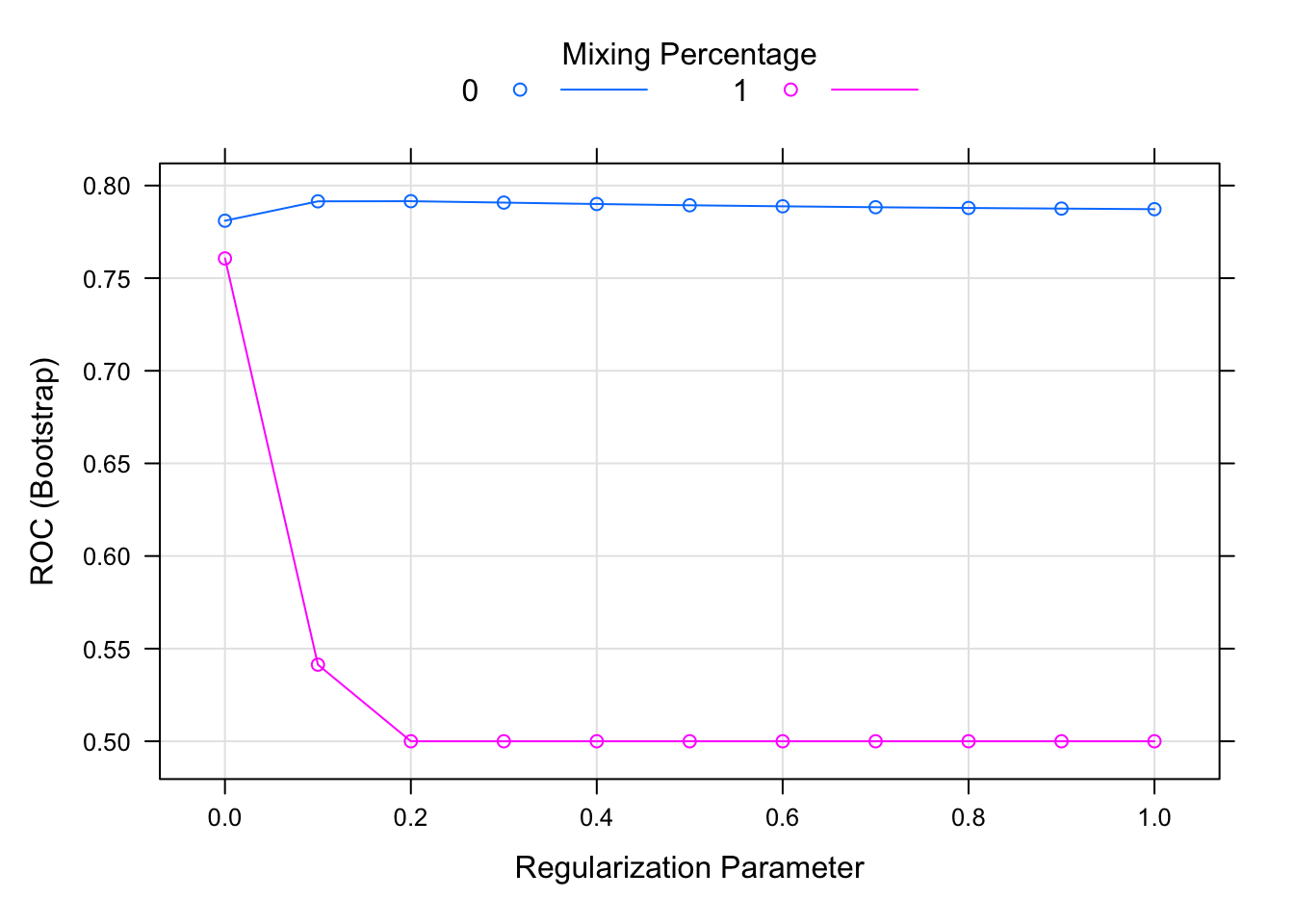
##   alpha  lambda  ROC        Sens        
##   0      0.0     0.7810206  0.2301791801
##   0      0.1     0.7914828  0.0654123018
##   0      0.2     0.7915574  0.0180324588
##   0      0.3     0.7907987  0.0067194096
##   0      0.4     0.7900281  0.0003533569
##   0      0.5     0.7893529  0.0000000000
##   0      0.6     0.7887966  0.0000000000
##   0      0.7     0.7883022  0.0000000000
##   0      0.8     0.7878990  0.0000000000
##   0      0.9     0.7875657  0.0000000000
##   0      1.0     0.7872430  0.0000000000
##   1      0.0     0.7606466  0.2673122987
##   1      0.1     0.5413578  0.0000000000
##   1      0.2     0.5000000  0.0000000000
##   1      0.3     0.5000000  0.0000000000
##   1      0.4     0.5000000  0.0000000000
##   1      0.5     0.5000000  0.0000000000
##   1      0.6     0.5000000  0.0000000000
##   1      0.7     0.5000000  0.0000000000
##   1      0.8     0.5000000  0.0000000000
##   1      0.9     0.5000000  0.0000000000
##   1      1.0     0.5000000  0.0000000000
##   Spec     
##   0.9685529
##   0.9957487
##   0.9996506
##   1.0000000
##   1.0000000
##   1.0000000
##   1.0000000
##   1.0000000
##   1.0000000
##   1.0000000
##   1.0000000
##   0.9584782
##   1.0000000
##   1.0000000
##   1.0000000
##   1.0000000
##   1.0000000
##   1.0000000
##   1.0000000
##   1.0000000
##   1.0000000
##   1.0000000
## 
## ROC was used to select the optimal
##  model using the largest value.
## The final values used for the model
##  were alpha = 0 and lambda = 0.2.

plot(glm_model)